Graph all the things

analyzing all the things you forgot to wonder about

Humans versus Zombies

2015-10-09
interests: game theory, cool plots

A friend and former college Humans vs. Zombies (HvZ) moderator gave me this problem: suppose we set up a game where an equal number of humans and zombies can disperse among 3 battlefields, and whichever faction wins on at least 2 battlefields is the overall winner. To simplify things, each team has the same number of total players, and each battle is won by the team with more players on that battlefield. What is the optimal way to allocate your players?

Every allocation is beaten by some other allocation. For instance, if I send my people equally to all battles $(\frac13, \frac13, \frac13)$ , my opponent can win with $(\frac12, \frac12, 0)$ . That strategy in turn could be beaten by $(0, \frac34, \frac14)$ , which is beaten by $(\frac13, \frac13, \frac13)$ .

I solved the game numerically, and here's what the solution looks like:

Beautiful probability density heat map on an equilateral triangle between the points (0, 0, 1), (0, 1, 0), and (1, 0, 0). The inner hexagram's edges are high-probability, and the outer subtriangles have no probability.

It's pretty cool, but let's first learn rock, paper, scissors.

Rock, Paper, Scissors (RPS)

In RPS, rock beats scissors, scissors beats paper, and paper beats rock. You get one point for beating the other person's choice, 1/2 a point for choosing the same thing, and 0 points for getting beaten.

I have a friend Mimee (who also helped me think through part of this problem) whose RPS strategy is to always play rock. This is great against anyone predisposed to play scissors, but doesn't work very well after people catch on. You can beat this strategy 100% of the time by playing paper.

My favorite strategy is to play whatever the other person's previous play would have beat. This works remarkably well against many people because they rarely play the same thing twice in a row. But arguably it still isn't a very good strategy - it would lose about 100% of the time to a stubborn person who keeps playing rock.

For competitive play, the best technique is of course to choose randomly, with equal probability given to rock, paper, and scissors. This way, no matter what technique the opponent uses, they can't get more points than you on average. Also, if both players use this strategy, neither can tweak their strategy to gain more points on average. This is known as a Nash Equilibrium!

In general, if your chances of playing rock, paper, or scissors are $x_r, x_p, x_s$ respectively, you have an expected outcome of $x_p + \frac12 x_r$ against someone playing rock, and so forth. This can be simply written as

$\begin{bmatrix} 0.5 & 1 & 0 \\ 0 & 0.5 & 1 \\ 1 & 0 & 0.5 \end{bmatrix} \begin{bmatrix} x_r \\ x_p \\ x_s \end{bmatrix} = \begin{bmatrix} y_r \\ y_p \\ y_s \end{bmatrix}$

where $y_r$ is your expected number of points against rock, and so forth. We can derive the optimal technique by demanding that we average at least 0.5 points; that $y_r, y_p, y_s \ge 0.5$ . If we don't, the opponent could average more points by always playing what we lose to on average. If we do, the opponent can't beat us more than 50% of the time regardless of their technique.

Generalizing RPS

We can easily generalize this problem. Suppose there are $i = 1, 2, 3, \ldots n$ possible plays, and play $j$ always has probability $a_{ij}$ to beat play $i$ . Then if we choose to make play $i$ with probability $x_i$ , our expected number of points against each opponent's play can be written as

$\begin{bmatrix}a_{11} & a_{12} & \ldots & a_{1n} \\ a_{21} & a_{22} & \ldots & a_{2n} \\ \vdots & \vdots & \ddots & \vdots \\ a_{n1} & a_{n2} & \ldots & a_{nn}\end{bmatrix}\begin{bmatrix}x_1 \\ x_2 \\ \vdots \\ x_n\end{bmatrix} = \begin{bmatrix}y_1 \\ y_2 \\ \vdots \\ y_n\end{bmatrix}$

Each $a_{ii}$ must be $1/2$ and each $a_{ij} + a_{ji} = 1$ . To write that more concisely, if this matrix is $A$ , then $A = 1-A^T$ . It would be nice to just let $\vec{y} = \vec{1/2}$ and invert $A$ to find the probability vector $\vec{x}$ we need to win half the time.

For example, if I modify RPS so that paper beats rock 80% of the time, scissors beat paper 60% of the time, and rock beats scissors 70% of the time, then the ideal strategy is to use $x_r = 1/6, x_p = 1/3, x_s = 1/2$ , which is obtained by inverting the matrix. Unfortunately, the solution is not always so simple.

First of all, there might be no solution for $\vec{x}$ to $A\vec{x} = \vec{1/2}$ . That's not to stay there is no best strategy, you just might not beat everything with exactly 50% probability. For instance, if we add in a useless fourth play (eye?) to RPS which loses to everything else, then inverting the matrix tells us to play eye with negative probability, which of course cannot be done. The best strategy is to play the original 3 plays with equal probability, which beats eye 100% of the time rather than 50%.

Second of all, there might be too many solutions (if the matrix is not invertible). For instance, if we add a fourth play (anti-rock?) to RPS which draws with rock, beats paper, and loses to scissors, then the normal RPS technique is optimal, but you can also incorporate anti-rock into your technique and still be optimal.

Using the existence of a Nash equilibrium, it is easy to show that there must exist a strategy in these symmetrics games giving at least $1/2$ points on average against any other play. Nash proved long ago that a Nash equilibrium exists for any finite game, and generalizations exist for many types of infinite games too (including our HvZ problem). Since such an equilibrium exists, consider the case when two players use it. Our game is symmetric with points summing to 1, so each player must get $1/2$ points on average. By definition of a Nash equilibrium, neither player can get more points by switching to a different strategy. Therefore there is no single play that beats the Nash equilibrium strategy on average. Proof complete!

The Solution

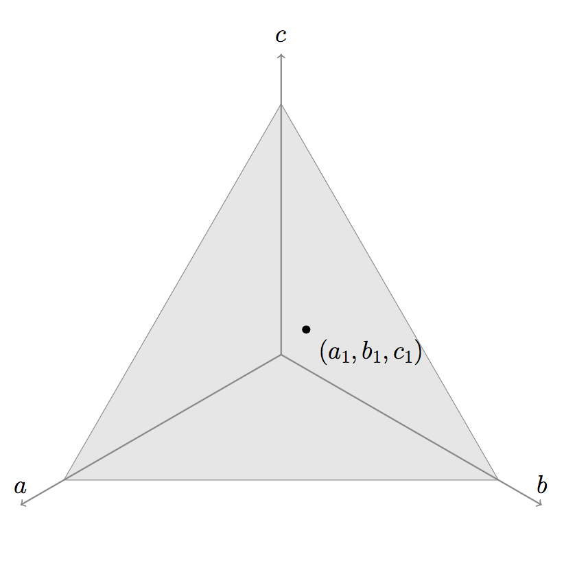
Returning to the HvZ problem, the infinite set of possible plays is a triangle in $(a, b, c)$ space defined by $a + b + c = 1, a \ge 0, b \ge 0, c \ge 0$ :

a point (a1, b1, c1) on the triangle between a, b, and c, each of which is a component vector

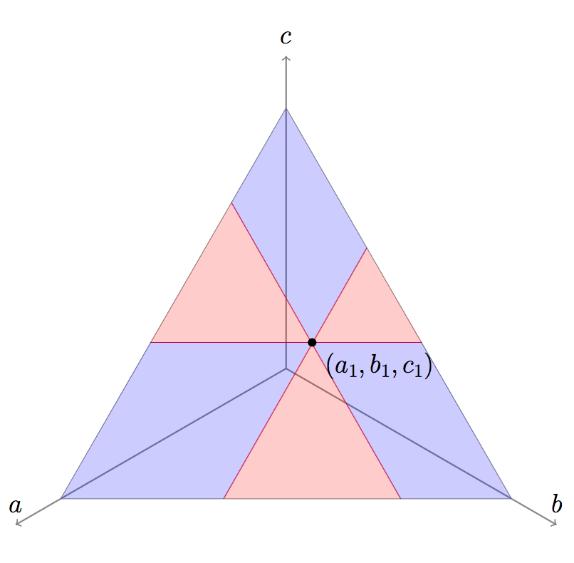
What plays does $(a_1, b_1, c_1)$ beat? Any play with $a_2 > a_1, b_2 < b_1,$ and $c_2 < c_1$ would work. Similarly if $a_2 < a_1, b_2 > b_1,$ and $c_2 < c_1$ ; or $a_2 < a_1, b_2 < b_1,$ and $c_2 > c_1$ . Plotting these possibilities, where the things $(a_1, b_1, c_1)$ beats are in blue, makes it a lot clearer what beats what:

that same triangle colored in 6 sections alternating between beating (a1, b1, c1) and being beaten by it

If we discretize this problem, it becomes a generalized RPS game; each play in the space has a probability to beat each other play in the space (either 0, 1/2, or 1). The full problem is just a continuous version of the discrete games we were considering earlier.

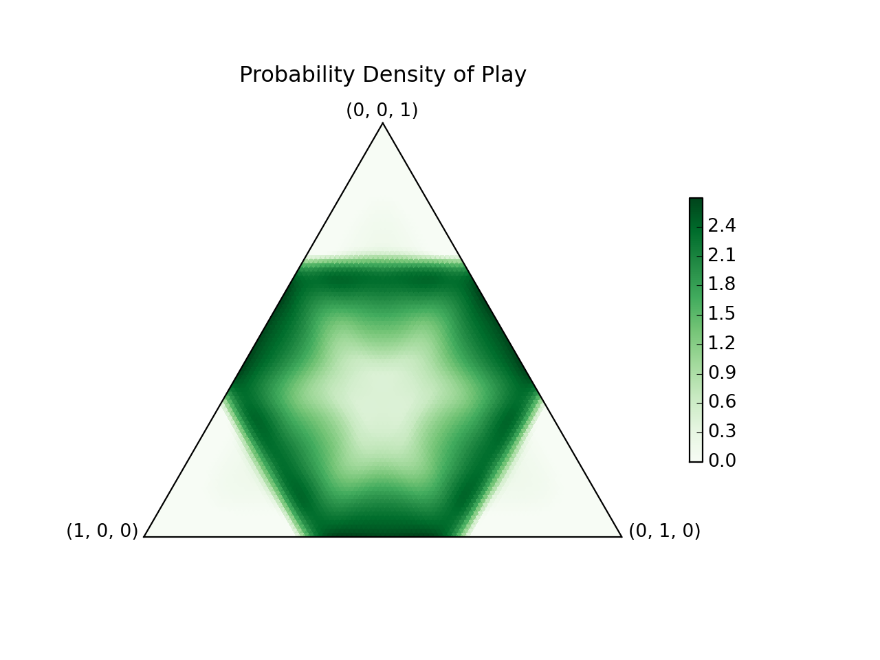
I wrote a numerical algorithm which efficiently converged to the solution. The optimum strategy is to sample from this probability density function over the set of plays:

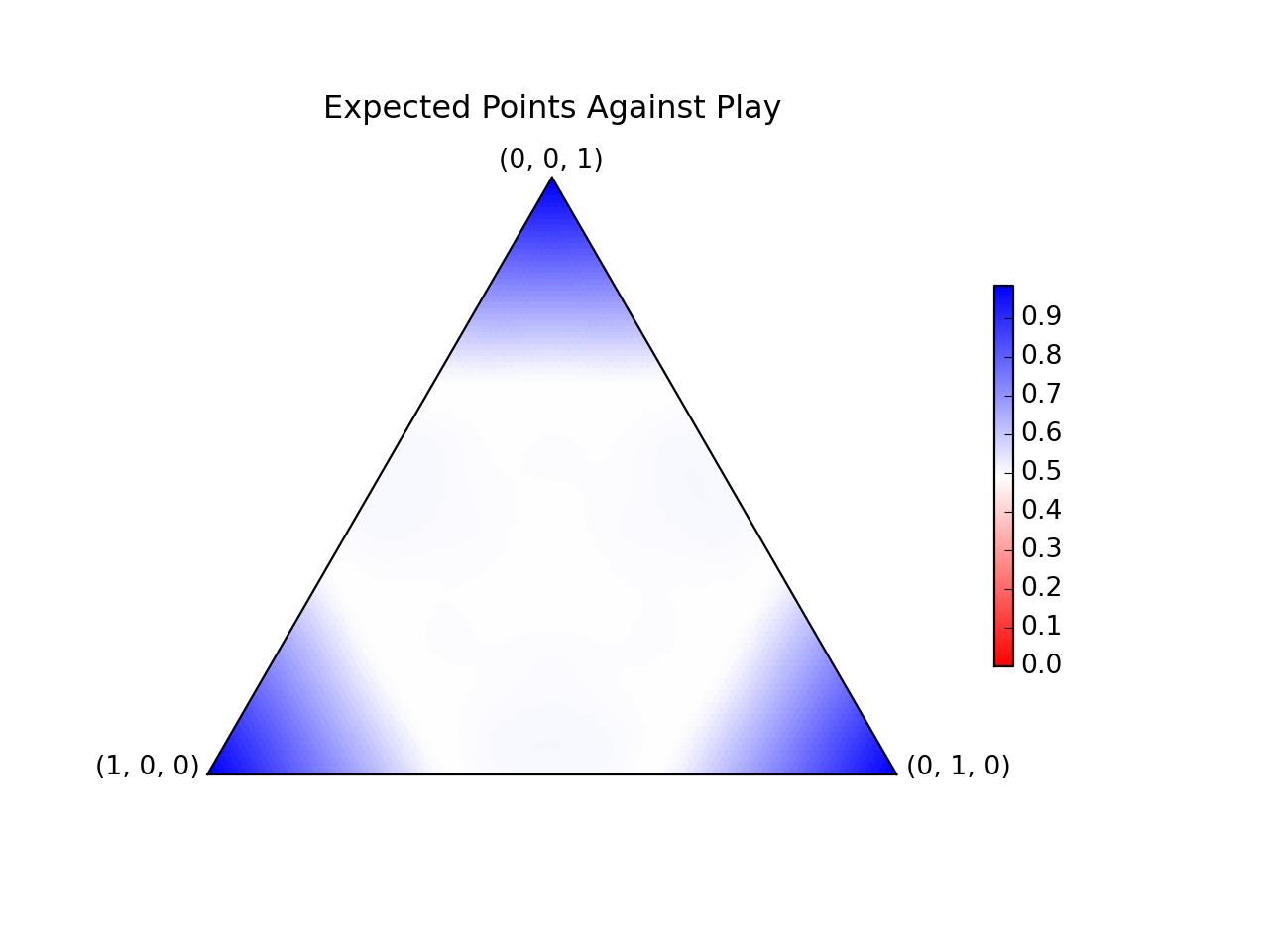
Wow! It's actually really pretty! Basically, play frequently near the edges of the main hexagon, with occasional forays into its interior. This wins against each possible play in the interior with 50% probability, and near the corners with more:

A plot on the equilateral triangle of expected points the optimal strategy gets against the play. The middle hexagon has 0.5 expected points, and the outer subtriangles have higher.

The numerical method works by discretizing the space into a triangular grid, then minimizing a cost function. Our goal is to not lose more than 50% of the time, so if the chance of beating each possible play is $y_{i,j}$ , my cost function is $L(y) = ||\max(0.5 - y, 0)||_2$ . I then applied a gradient descent algorithm to find the optimal probability $x_{i,j}$ of each play.

To account for the normalization (that $\sum_{i,j} x_{i,j} = 1$ ), I had the gradient descent take into account not only the change in each $y_{k,l}$ with respect to each $x_{i,j}$ , but also the incremental normalization on all coordinates that would be incurred by increasing any $x_{i,j}$ . Explicitly, this adds $-\sum_{i,j} \sum_{k,l} x_{i,j}\frac{\partial y_{k,l}}{\partial x_{i,j}}\frac{\partial E}{\partial y_{k,l}}$ to each gradient. Without taking this geometry of the problem into account (by just doing dumb gradient descent without constraints), the algorithm did not even converge to the right solution. I coded the right algorithm in a computationally efficient manner.

Closing Thoughts

I'm probably never going to play RPS, or this HvZ problem, using the optimum strategy. It's no fun to win half the time regardless of what the other person does.

Update: Analytic Solution

This is apparently a case of the continuous Colonel Blotto game, and two researchers pretty much solved it in this 2006 working paper. The hexagon strategy shown here is a real solution, but there are additional solutions in which you play on smaller hexagons near the vertices of that hexagon, or yet smaller hexagons near the vertices of those hexagons, and so forth. I think that's interesting, because as you use smaller and smaller hexagons, the total area of the support of your strategy shrinks to 0; you are playing on a type of Cantor set.

< previous next >