Graph all the things

analyzing all the things you forgot to wonder about

Traffic

2015-01-10
interests: traffic (skim for the results), PDEs

If you have learned to drive, your instructor may have told you to obey the "2-second rule", which states that you should drive such that your car is always 2 seconds behind the car ahead of you. It turns out that if everyone were obey this exactly, traffic jams would rarely ever disappear. Fortunately, there is a solution: if everyone adjusts their time to the next car based on their speed as in the following chart, traffic jams will dissipate more quickly. More modern suggestions for these times made from a safety standpoint match up closely.

Speed/(km/hr)	Speed/mph	Time to next car/seconds
0-30	0-19	1
31-62	20-39	2
63-100	40-63	3
101-143	64-90	4

The only discrepancy is that you may want to stay 2 seconds away even at very low speed. Please don't do anything stupid just because of this post.

Gamma

If you follow some sort of " $n$ -second rule" exactly, your distance to the next car is proportional to your speed. This rule makes sense if you are expecting to slow down, say, 20 km/hr if something unexpected happens, but the distance required to stop your car entirely is proportional to the square of your speed instead. For practical purposes, you might pick some rule where your distance to the next car is

$d=Cv^{\gamma}$

Where $v$ is your speed and $C$ and $\gamma$ are (nonnegative) constants.

I'm going to analyze some partial differential equations (PDEs) here, so if you aren't comfortable, feel free to skip to the plots - just make sure you understand that $\gamma$ determines how you scale your distance to the next car with speed.

$\gamma=$ 0 or 1 cases

For simplicity, let's make the following assumptions: Everyone obeys $d=Cv^\gamma$ for some constant $\gamma$ and some $C$ . For most of this post, I'll assume everyone uses the same $C$ . The road is infinitely long. Everyone's speed is high enough that a car length is small compared to their distance to the next car (that means I'm only considering traffic jams where people slow down, not stop). As with most traffic setups, the flux of cars through a particular section of road is

$\Phi=\rho v$

where $\rho$ is traffic density (in, say, cars/km) and $v$ is their speed in that section. The rate of change in traffic density with time there is

$\rho_t=-\Phi_x$

where $x$ is distance along the road. The simplest case is $\gamma=0$ . That means that each car stays a constant distance from the car in front of it, regardless of speed - a terrible policy in real life. A driver's velocity would then be the same as the that of the driver in front of him, so every car has the same speed. This implies $v$ does not depend on $x$ , so $\rho_t = -v\rho_x$ . This is just a transport equation whose solution looks like this:

gif of traffic density moving forward as time passes

Here, the green dots represent particular cars as they move with the traffic. The shape of the traffic density is entirely determined by the initial condition of the road - it could be any other function, but it (and the cars) would still move in unison. However, this ubiquitous velocity could vary with time, so the problem has many possible solutions; it is not well-posed. We could observe all the cars speeding up or slowing down, as long as it was done in unison.

Since I just dealt with the case $\gamma=0$ , I'm going to assume $\gamma>0$ for the rest of this post. These cases are more complicated, so until the end of the post I will also assume that each driver uses the same constant $C$ . We know that $d$ is inversely proportional to the traffic density $\rho$ , so

$v=k\rho^{-1/\gamma}$

for some universal constant $k$ . This brings me to the second simple case: $\gamma=1$ . That means $\Phi=k$ , so $\rho_t=0$ . In other words, the traffic stays in place while the cars move:

gif of traffic density staying in place as time passes, with individual cars moving forward

General $\gamma$ case

In the case that $\gamma$ is arbitrary but $k$ is constant, our equations give $v=k\rho^{-1/\gamma}$ , which in turn means that the flux is

$\Phi=k\rho^{1-1/\gamma}$

That means our partial differential equation is

$\rho_t + \left(k\rho^{1-1/\gamma}\right)_x = 0$

This is a type of Burger's equation whose properties are fairly well-understood. This equation describes the traffic moving at

$v_{\text{traffic}}=k\left(1-\frac1\gamma\right)\rho^{-1/\gamma}$

whereas the individual cars move at speed

$v=k\rho^{-1/\gamma}$

by definition. This is agrees with our example with $\gamma=1$ above, where the traffic did not move at all. For $\gamma< 1$ , we will observe the traffic density moving backwards as cars go forward, and for $\gamma>1$ , the traffic density will move forward.

Solving this PDE is difficult since discontinuities appear when fast traffic and slow traffic meet, causing a shockwave. Here's an example of a shockwave forming with $\gamma=2$ :

gif of a low-traffic area catching up with a high-traffic area as both move forward

There is of course a physically acceptable solution after this discontinuity occurs - one in which the number of cars is conserved (the entropy condition). The discontinuity remains, moving at speed

$v_\text{shock}=k\frac{\rho_r^{1-1/\gamma}-\rho_\ell^{1-1/\gamma}}{\rho_r-\rho_\ell}$

where $\rho_r$ is the traffic density on the right of the shockwave and $\rho_\ell$ is the density on the left. In the example above, that speed is $4/3$ , which is somewhere between the speed of the fast traffic density and the slow traffic density. As alluded to before, the shock will move backward in the case that $\gamma=1/2$ . This actually happens in real life when cars stop within the jam (https://www.youtube.com/watch?v=7wm-pZp_mi0). Here's an animation:

gif of a high-traffic area and low-traffic area running into each other as both move backwards

This may appear to be the mirror image of the $\gamma=2$ , case, but they are algebraically different. An algebraically similar situation actually arises when slow traffic follows fast traffic. This results in a sort of anti-shock where slow cars need to accelerate to fill in the growing gap between them and the fast cars, as seen in the next animation.

Fortunately, traffic jams ultimately dissipate as long as $\gamma$ is not 0 or 1. While the jam is extending on one end, it is growing shorter on the other end at a faster rate. Here's an example with $\gamma=2$ :

gif of a small high-traffic area spreading out and becoming less severe as it moves forward

What would be the ideal $\gamma$ for eliminating traffic jams? For which $\gamma$ does the low traffic density "catch up" to the front of the traffic jam most quickly? You might have expected the answer: the smallest $\gamma$ possible. Unfortunately, this is a horrible idea unless you enjoy rear-ending everyone on the highway. If we only seriously consider $\gamma>1$ , the question gets interesting.

Remarkably, the best safe $\gamma$ is always between 1 and 2. Take a look at this example where the traffic density in the jam is twice as high as normal:

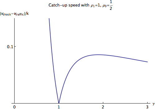
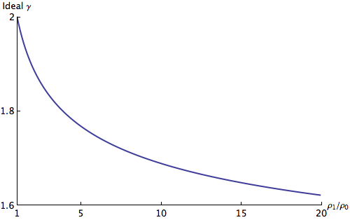
plot of catch-up speed versus gamma, dipping sharply to 0 as gamma reaches 1, then rising up again and peaking around gamma of 1.7

The denser the jam relative to the rest of the traffic, the lower $\gamma$ should be. I'd say we can reasonably expect the density ratio $\rho_1/\rho_0$ to be no more than 20, and in those cases, the best $\gamma$ is actually between 1.6 and 2. The catch-up speed is a fairly flat function of $\gamma$ in that interval anyway, so any $\gamma$ in that range will do. If you want to be picky, here's the optimal $\gamma$ as a function of $\rho_1/\rho_0$ :

plot of ideal gamma versus rho 1 / rho 0

In general, I think $\gamma=1.7$ is reasonable. That's what I used to make the chart at the top, along with the 3-second rule at 80 km/hr.

Here's the caveat: for $\gamma>1$ , a short traffic jam slows down each driver less than a long section of slightly increased traffic. So why would we even want to dissipate traffic jams? The answer is the speed limit. If we enforce a speed limit, no matter how sparse the traffic becomes, no one will exceed a certain speed; if traffic is only slightly increased in one region, no one would have to slow down at all. This tends to be the case in reality, so long sections of slightly denser traffic usually cause little impedance.

More things to explore

If $C$ differs from car to car, then $k$ does as well, and it propagates at the same speed as the cars. That implies

$k_t +k\rho^{-1/\gamma}k_x = 0$

$p_t +\left(k\rho^{1-1/\gamma}\right)_x = 0$

This is an abominable system of nonlinear partial differential equations. I plan on making a numerical method for this and animating some scenarios in a future post.

I also didn't have space to animate the effect of a speed limit on traffic, so I'll include that as well.

< previous next >

Traffic

Gamma

0 or 1 cases

General case

More things to explore

$\gamma=$ 0 or 1 cases

General $\gamma$ case