Graph all the things

analyzing all the things you forgot to wonder about

President Rankings

2017-05-11
interests: US history, unsupervised learning, interactive visualizations

Some historians find it fun to rank presidents, and they do this regularly in the Sienna Research Institute Presidents Study, ranking all past presidents on 20 different criteria. I noticed that the rankings are heavily redundant. Just look at "overall ability" versus "executive ability" - that's 96% correlation! To make a bit more sense of this 20-dimensional data (a ranking for each category for each president), I plotted each president's rankings in 20-dimensional space, then rotated and recentered them so that the axes line up with the directions the data varies in.

Click on a president to follow him, and compare different axes!

Factors the x axis (component 1) is positively and negatively affected by:

expert view,

executive ability,

overall ability,

domestic policy,

leadership,

imagination,

executive appointments,

communication,

court appointments,

handling of economy,

relations with congress,

willing to take risks,

foreign policy,

intelligence,

avoid crucial mistakes,

party leadership,

ability to compromise,

luck,

integrity,

background

Factors the y axis (component 2) is positively and negatively affected by:

background,

intelligence,

integrity,

court appointments,

executive appointments,

overall ability,

imagination,

foreign policy,

expert view,

handling of economy,

executive ability,

domestic policy,

communication,

avoid crucial mistakes,

ability to compromise,

leadership,

willing to take risks,

party leadership,

relations with congress,

luck

This is called Principal Component Analysis (PCA). The resulting dimensions are ranked from most to least descriptive, and the first (most descriptive) one is called the principal component.

My takeaways from this are:

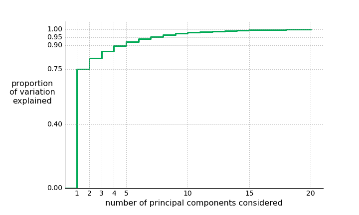
The most descriptive quality for a president is how good they generally were. This axis alone explains 75% of the dataset's variation.
The 2nd most descriptive quality for a president is how much more redeeming their qualities were than their successes.
The 3rd most descriptive quality for a president is the extent to which they made cautious (and ethical) decisions without collaboration/leadership.
The 4th most descriptive quality for a president is the extent to which they made cautious decisions with collaboration/leadership.
Any components after that are either too hard to interpret or basically just noise; the remaining 16 only constitute 10% of the dataset's variation. Perhaps these first 4 components are the only true criteria we should bother asking historians.
Lyndon B. Johnson is the most interesting president.

Here's the proportion of the data that's conveyed by the first $k$ components:

proportion of variance explained versus number of principal components considered

Math and Intuition for PCA

This part relies on knowledge of covariance and basic linear algebra.

Let $(X_1, \ldots X_n) = X$ be a random variable in $\mathbb{R}^n$ with $n\times n$ covariance matrix $A$ (in this case, $n=20$ and the variables are the rankings, so the covariance is Spearman's rank covariance). The principal components of the probability distribution are the normalized eigenvectors $v_1, \ldots v_n$ of $A$ . They have important properties that make PCA meaningful:

The most descriptive component is the one with the largest corresponding eigenvalue. In general, the eigenvalue $\lambda_i$ corresponding to $v_i$ is the variance of the distribution of $X$ in the direction of $v_i$ ; that is, $\lambda_i = \text{Var}[v_i \cdot X]$ . This gives a nice easy way to rank the components from most to least descriptive.
The principal components are uncorrelated; $\text{Cov}[v_i\cdot X, v_j\cdot X] = 0$ for $i\ne j$ . This is what makes the data appear to line up with the axes.

In fact, PCA can be derived from that last bullet. If you remember some basic formulas for covariance,

$\text{Cov}[v_i\cdot X, v_j\cdot X] = \sum_{k=1}^n\sum_{l=1}^nv_{ik}v_{il}\text{Cov}[X_k, X_l]$

$\text{Cov}[v_i\cdot X, v_j\cdot X] = \sum_{k=1}^n\sum_{l=1}^nv_{ik}v_{il}A_{kl}$

$\text{Cov}[v_i\cdot X, v_j\cdot X] = v_i^TAv_j$

Since we must have $\text{Cov}[v_i\cdot X, v_j\cdot X] = 0$ for $i\ne j$ , the uncorrelated components we are looking for must be orthogonal under the covariance matrix $A$ . Since all covariance matrices are positive definite, that condition is uniquely satisfied (up to scaling) by the eigenectors of $A$ . And if we use the normalized eigenvectors, we get

$\text{Var}[v_i\cdot X] = v_i^TAv_i$

$\text{Var}[v_i\cdot X] = \lambda_iv_i^Tv_i$

$\text{Var}[v_i\cdot X] = \lambda_i$

which gives us that nice easy way to order the components by importance like I mentioned earlier.

< previous next >